What is Multi-horizon Forecasting?
Multi-horizon forecasting means, forecasting multiple future values for given input values. You can call this multi-step-ahead forecasting too.
(e.g. predicting daily market demand for the next 7 days)
Before the multi-step-ahead forecasting, let’s take a brief look at the concept of one-step-ahead forecasting first. In the simplest case of univariate data, it can be represented as:
$$ \hat{y}_{t+1} = f(y_{t-k:t}, \textbf{x}_{t-k:t}, \textbf{s}) $$
Here, \( y_{t-k:t} = \{ y_{t-k}, … ,y_t \} \) and \( \textbf{x}_{t-k:t} = \{ \textbf{x}_{t-k}, … , \textbf{x}_t \} \) are observations of the target and exogenous inputs respectively, over a look-back window \( k \), \( s \) is static metadata of the entity (e.g. user profile), and \( f(.) \) is the model.
Namely, the objective of the model is to predict \( y_{t+1} \).
Actually, multi-horizon forecasting is nothing more than a slight modification of one-step-ahead prediction, as below:
$$ \hat{y}_{t+\tau} = f(y_{t-k:t}, \textbf{x}_{t-k:t}, \textbf{u}_{t-k:t+\tau}, \textbf{s}, \tau) $$
- \( \tau \in \{ 1, … , \tau_{max} \} \) is a discrete forecast horizon, which means the model is required to predict from \( y_{t+1} \) to \( y_{t+\tau} \).
- \( \textbf{u}_t \) are known future inputs (e.g. day-of-week or month information) across the entire horizon.
- \( \textbf{x}_t \) are inputs that can only be observed historically.
Generally, there are two types of methods for multi-horizon forecasting: iterative methods vs. direct methods.
Iterative Methods vs. Direct Methods
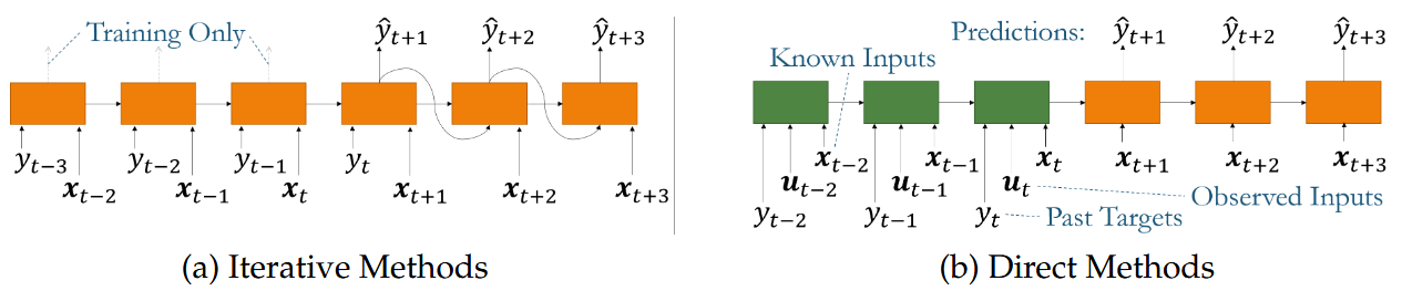
1. Iterative Methods
- In iterative forecasting, the model is trained to predict only a single step ahead (\( y_{t+1} \)).
- To generate multi-step-ahead forecasts, the model recursively uses its own predictions as inputs for the next step.
- This is similar to how traditional autoregressive (AR) models work.
Advantages
- Can leverage standard deep learning models trained for one-step forecasting.
- Works well when dependencies between time steps are strong.
Disadvantages
- Error accumulation: Small prediction errors compound over multiple steps, leading to poor long-horizon forecasts.
- Instability: Since the model relies on its own generated predictions, feedback loops can amplify errors.
2. Direct Methods
- Instead of predicting one step ahead and iterating, direct methods train a separate model (or output layer) for each step ahead.
- For example:
- A model could be trained to predict \( y_{t+1} \).
- Another model (or separate output) predicts \( y_{t+2} \), and so on.
- In deep learning implementations, this can be done using multi-output networks, where a single model outputs multiple future values at once.
Advantages
- No error accumulation: Since each step is predicted independently, errors do not propagate recursively.
- Better stability for long-term forecasting.
Disadvantages
- Requires significantly more training data because each step needs a separate model or specialized network output.
- Can be computationally expensive as more models (or complex architectures) are needed.
Then.. which one is better?
- For short-term forecasting, iterative methods are often preferable due to their simplicity and efficiency.
- For long-term forecasting, direct methods typically perform better since they avoid error accumulation.
In practice, hybrid approaches combining both methods have been explored, such as sequence-to-sequence (Seq2Seq) models that balance both strategies effectively.
Reference: Time Series Forecasting With Deep Learning: A Survey